7 Basic Symbolization of Vector Data
One of the main powers of any GIS lies in its ability to present spatial data visually. When working with vector data, it is important to utilize schemes that best communicate your message, while making the data clear and understandable. This is a basic element of Cartography, or the study of making maps.
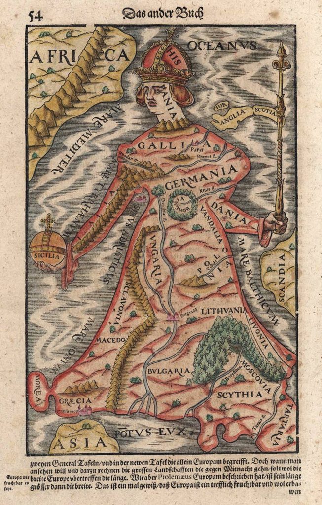
The early map, depicted in figure 1, was symbolized to send a very poignant message. As you choose which colors, and schemes, to use, be mindful of the intended audience and what you hope to convey. Be ethical in how you symbolize your data as maps can be a powerful tool to sway opinions!
Although GEE’s main strength is the ability to display, and analyze, large datasets, we may want to customize how we visualize things. Let’s look at an example to create, and display, a point for Brno, the second largest city in the Czech Republic:
Example 2.4
- var lat = 49.1951;
- var lon = 16.6068;
- var Brno = ee.Geometry.Point(lon,lat);
- Map.addLayer(Brno);
- Map.centerObject(Brno,7.8);
There’s nothing new in the script above. After running, you see Brno appear on the map, indicated by a small black dot. Inspecting the layers allows you to toggle the point on and off again. Let’s assume we want the Brno point to be a different color, say red, and give it a name ‘Brno’. To do this, we need to pass arguments into Map.addLayer():
Example 2.5. Changes from 2.4 highlighted in Bold.
- var lat = 49.1951;
- var lon = 16.6068;
- var Brno = ee.Geometry.Point(lon,lat);
- Map.addLayer(Brno, {color:’red’}, ‘Brno’);
- Map.centerObject(Brno,7.8);
After running this script, you see the point changes color. You might note the curly brackets encompassing color:’red’. Remember what this is? This is an object. Map.addLayer() expects, within its brackets the following:
Map.addLayer(the layer to be added, visual parameters, name of the layer to be displayed).
It is often useful to separate these visual parameters into its own variable:
Example 2.6.
- var lat = 49.1951;
- var lon = 16.6068;
- //Create a point for Brno
- var Brno = ee.Geometry.Point(lon,lat);
- //Create a variable, point_vis_params, for the way it will be displayed
- var point_vis_params = {
- color:’red’,
- };
- //Display the data
- Map.addLayer(Brno, point_vis_params,’Brno’);
- Map.centerObject(Brno,7.8);
In this particular case, this doesn’t really simplify things. However, as we build into rasters, you will see there are many more elements that need to be defined to properly display imagery. It also helps in organizing your script.
Now, try to add the Czech Republic to the map using the LSIB_SIMPLE county boundary dataset. Please note: the country name is found as “Czechia”. Create an object called “area_vis_params” to make the country the color you would like. Here’s my solution:
Example 2.7.
- var lat = 49.1951;
- var lon = 16.6068;
- var Brno = ee.Geometry.Point(lon,lat);
- var point_vis_params = {
- color:’red’
- };
- var Czechia = ee.FeatureCollection(‘USDOS/LSIB_SIMPLE/2017’).filter(‘country_na==”Czechia”‘);
- var area_vis_params = {
- color:’black’
- };
- Map.addLayer(Czechia,area_vis_params,’Czech Republic’);
- Map.addLayer(Brno, point_vis_params,’Brno’);
- Map.centerObject(Brno,7.8);
Later you’ll see how to create palettes to display unique values within a dataset. For now, this is sufficient.
In the next chapter, we’ll change gears. We’ve really only dealt with vector data here. We’ve created some points and we’ve displayed some polygons. It doesn’t take a supercomputer to do this. However, it might take a supercomputer to analyze that data over a wide area. For the most part, we really want to use vector data to compliment rasters, or imagery. Imagery, especially that of high spectral and spatial resolution, is massive. It’s difficult to analyze even a small portion of the world without utilizing some serious graphical and computational processors. This is where GEE shines. Although we can use our own assets, GEE also contains a wide variety of current, and historical raster data. This includes the very popular Landsat and Sentinel data sets. The remainder of this part of the book is designed to introduce you to using the data library to find, and filter, raster data sets from the data catalog.
